Here we describe a practical example from research based here in Cardiff.
We have used Bayesian Nets in a Computer Vision application. Details of the visual processes involved will be discussed later in the course so the contest will become clearer later.
Here we attempt to describe the Bayesian reasoning behind the process.
The goal is to perform a task called data fusion to obtain a segmentation -- a description of an object (viewed from a set of images) detailing its surface properties. In the example given here we deal with a simple cube. So the final description will hopefully list its edges and its faces and how they are connected together.
The input to the fusion process is three preprocessing stages that have extracted out edge information and planar surface information from 2D grey scale (monochrome) images and 3D range data.
So from these three pre-processes we have a list of all lines, curved or straight, a list of all line intersections (two or three line intersections) and a list of all the surface equations extracted from both image types. We can now build the network from these lists of features. As mentioned above, we hypothesise about extracted surfaces intersecting. For us to evaluate these hypotheses we need to have evidence to support or contradict them. The evidence that we use is :
The two lines lists are generated as described above. The areas of uncertainty are found when we are attempting to find the surface equations of each surface type. Errors are found in the depth map where the mask to find the general surface shape overlaps two or more surfaces, the error tends to be enlarged therefore, giving us a clue that a surface intersection exists in that general area. So we are using evidence from more than one source of data.
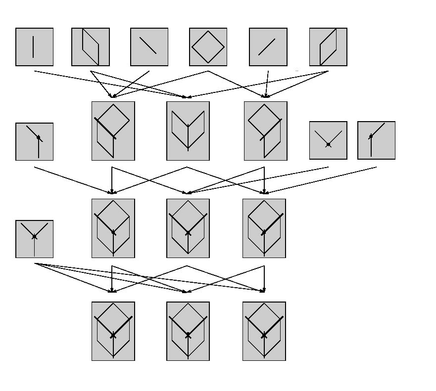
We proceed by taking each of the surfaces in the surface list and a node is generated to represent it. We then take a pair of surfaces and attempt to intersect them. If they are possibly intersecting then a `feature group' node is generated referencing the surfaces and connected to the children surface nodes. This process is repeated for each pair surfaces that we have extracted. We now want to attach a conditional probability to each of our new nodes. So we now know the surfaces that could possibly interact in the object. We now attach a probability to these connections. We do this by finding the equation of intersection, this will be a three dimensional line for two planes or an ellipse for a plane and a sphere, and project this onto our focal plane. Now we have our hypothesised intersections in the same dimension as our extracted lines from the preliminary stage. So we now find, for each intersecting line a closest match line from our line list. Once we have found the closest matching line we generate a probability from the error. So a line that closely matches our intersection line then we have a high probability whereas two surfaces that don't intersect in the object are unlikely to coincide with a line from the line list therefore giving us a low probability. The line that is found is also checked to see if it lies in an area of uncertainty. If it does then that is another strong clue that the line that we have found is actually where surfaces are joined.
So once we have generated this network with all the necessary links etc. any more information that is provided to the system can be added and the network will propagate this information throughout the network in the form of probability updating. So for example say a new image was provided from say a colour image and this image increased the likelihood of some edges and corners being present in the image then this would increase the probability of those features that are linked to those edges and corners which would propagate throughout the network. Figure 22 shows us a simple example of the network that would be generated from the input data of edges and planar faces of the cube. As can be seen, the feature group nodes can represent groups that vary from single features such as line segments, surfaces or corners or the whole object is represented in the lower nodes which includes three surfaces, three line segments, three crosses and one corner.

Fig. 22 A Bayesian Network for Segmentation of a Cube