The Fast Fourier Transform Algorithm

This is how the DFT may be computed efficiently.

1D Case

has to be evaluated for N values of u, which if done in the obvious way clearly takes multiplications.

It is possible to calculate the DFT more efficiently than this, using the fast Fourier transform or FFT algorithm, which reduces the number of operations to .

We shall assume for simplicity that N is a power of 2, .

If we define to be the root of unity given by , and set M=N/2, we have

This can be split apart into two separate sums of alternate terms from the original sum,

Now, since the square of a root of unity is an root of unity, we have that

and hence

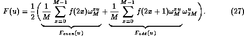
If we call the two sums demarcated above and respectively, then we have
 

Note that each of and for is in itself a discrete Fourier transform over N/2=M points.

How does this help us?

Well

and we can also write
 

Thus, we can compute an N-point DFT by dividing it into two parts:

• The first half of F(u) for can be found from Eqn. 28,
  
• The second half for can be found simply be reusing the same terms differently as shown by Eqn. 30.
  
• This is obviously a divide and conquer method.

To show how many operations this requires, let T(n) be the time taken to perform a transform of size , measured by the number of multiplications performed. The above analysis shows that
 
the first term on the right hand side coming from the two transforms of half the original size, and the second term coming from the multiplications of by . Induction can be used to prove that
 

A similar argument can also be applied to the number of additions required, to show that the algorithm as a whole takes time .

Also Note that the same algorithm can be used with a little modification to perform the inverse DFT too. Going back to the definitions of the DFT and its inverse,

and

If we take the complex conjugate of the second equation, we have that

This now looks (apart from a factor of 1/N) like a forward DFT, rather than an inverse DFT.

Thus to compute an inverse DFT,

• take the conjugate of the Fourier space data,
  
• put conjugate through a forward DFT algorithm,
  
• take the conjugate of the result, at the same time multiplying each value by N.

2D Case

The same fast Fourier transform algorithm can be used -- applying the separability property of the 2D transform.

Rewrite the 2D DFT as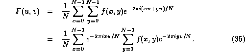

The right hand sum is basically just a one-dimensional DFT if x is held constant. The left hand sum is then another one-dimensional DFT performed with the numbers that come out of the first set of sums.

So we can compute a two-dimensional DFT by

• performing a one-dimensional DFT for each value of x, i.e. for each column of f(x,y), then
  
• performing a one-dimensional DFT in the opposite direction (for each row) on the resulting values.

This requires a total of 2 N one dimensional transforms, so the overall process takes time .